
Visualisation of covariate sensitivity analysis results
Source:R/sg-covsens-vis.R
sg_covsens_vis.RdDraw a forest-style graphic (points with uncertainty intervals) from the
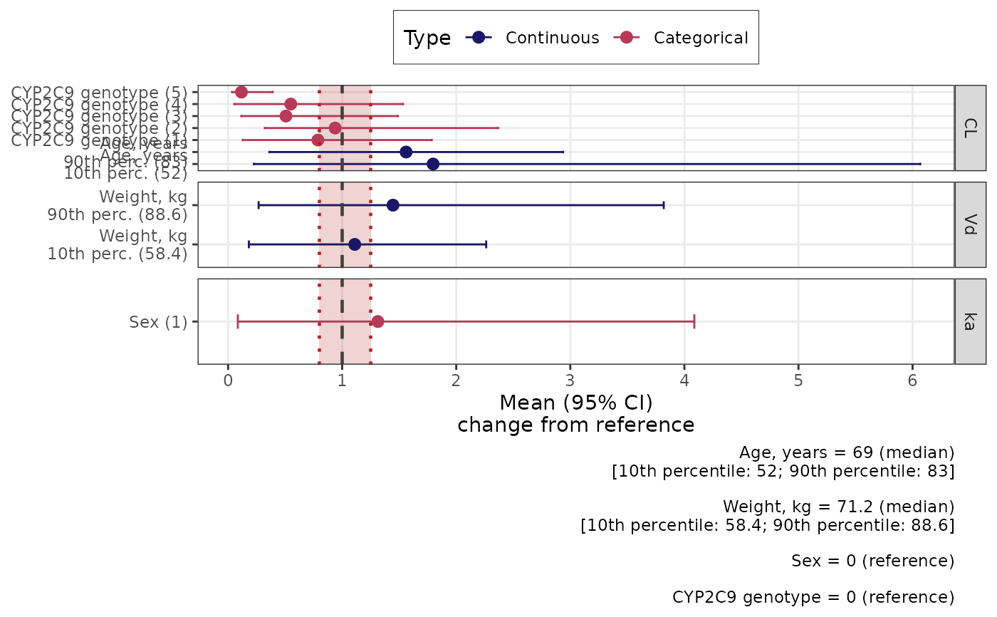
sensitivity tables produced by sg_covsens_sim. Each facet row
corresponds to a model output or exposure metric (VAR); each point is a
covariate scenario (LAB), coloured by covariate type (Type).
Usage
sg_covsens_vis(
  covsens_res,
  plot_type = c("PARSENS", "EXPSENS"),
  exclude_vars = NULL,
  ci = 95,
  ci_limits = c(0.8, 1.25),
  ci_band_alpha = 0.2,
  ci_band_col = "firebrick",
  ref_line_col = "grey25",
  palette = MSDcol[c(1, 3, 4, 5, 6, 7)],
  point_size = 2.5,
  errorbar_width = 0.2,
  lab_y = "standard",
  cap = "standard",
  var_nice_names = NULL
)
Arguments
- covsens_res
Named list as returned by
sg_covsens_sim(). Must contain the element selected bytype(PARSENSand/orEXPSENSdata.frames with columnsLAB,VAR,mean,Type, and the interval columns named byci_quantiles).- plot_type
Character scalar:
"PARSENS"(default) or"EXPSENS".- exclude_vars
Character vector. Contains
VARlevels to omit (e.g."Cc_Cmin").NULLkeeps all rows.- ci
Numeric. Confidence level in percents. Default is 95
- ci_limits
Numeric vector of length 2: lower and upper bounds of the shaded acceptance band and of the dotted horizontal guides. Default
c(0.8, 1.25)is a common bioequivalence-style window on the ratio scale.- ci_band_alpha
Numeric in \([0,1]\): transparency of the shaded band. Default
0.2.- ci_band_col
Color for the band fill and dotted limit lines. Default
"firebrick".- ref_line_col
Color for the dashed horizontal line at
y = 1(no change from reference). Default"grey25".- palette
Colors for the
Typescale (continuous vs categorical covariates, etc.). Recycled if there are more levels than colors. DefaultMSDcol[c(1, 3, 4, 5, 6, 7)].- point_size
Point size for
geom_point. Default2.5.- errorbar_width
Numeric. Width argument for
geom_errorbar. Default0.2.- lab_y
Axis label for the numeric scale (this becomes the horizontal axis after
coord_flip()). Default mentions a 95% interval; change if you use differentci_quantiles.- cap
Optional figure caption, passed to
ggplot2::labs(caption = ...)(e.g. text describing reference covariate values). DefaultNULL.- var_nice_names
Named character vector. Display labels for exposure facet rows when
plot_type = "EXPSENS". Names must match the unique values inVAR(afterexclude_vars); length equals the number of those unique values. DefaultNULL(facets useVAR).
Value
A ggplot2 object (inactive until printed or saved). You can
add further layers or themes with the usual ggplot2 API.
Details
Two views are available, matching the named elements of the simulation output:
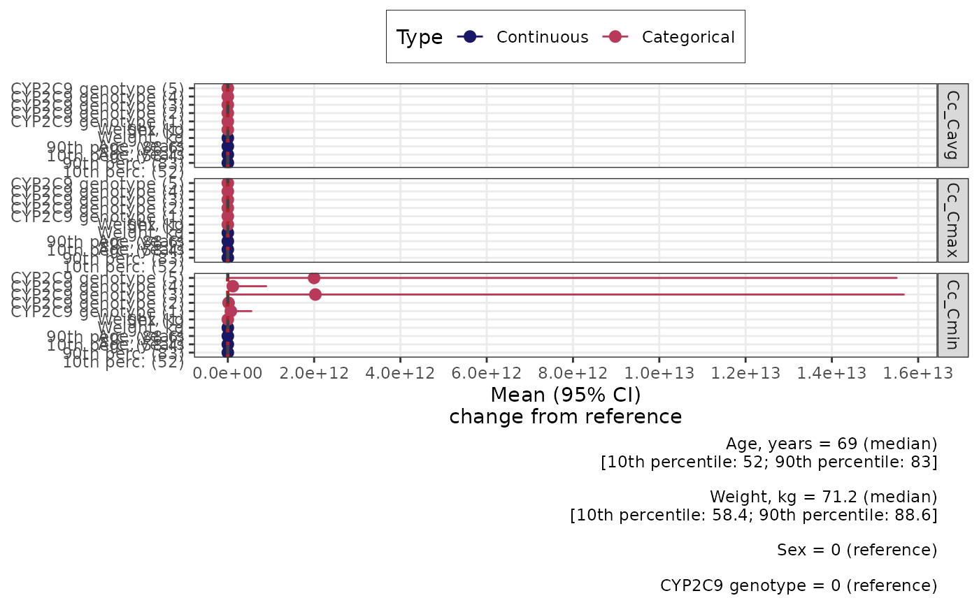
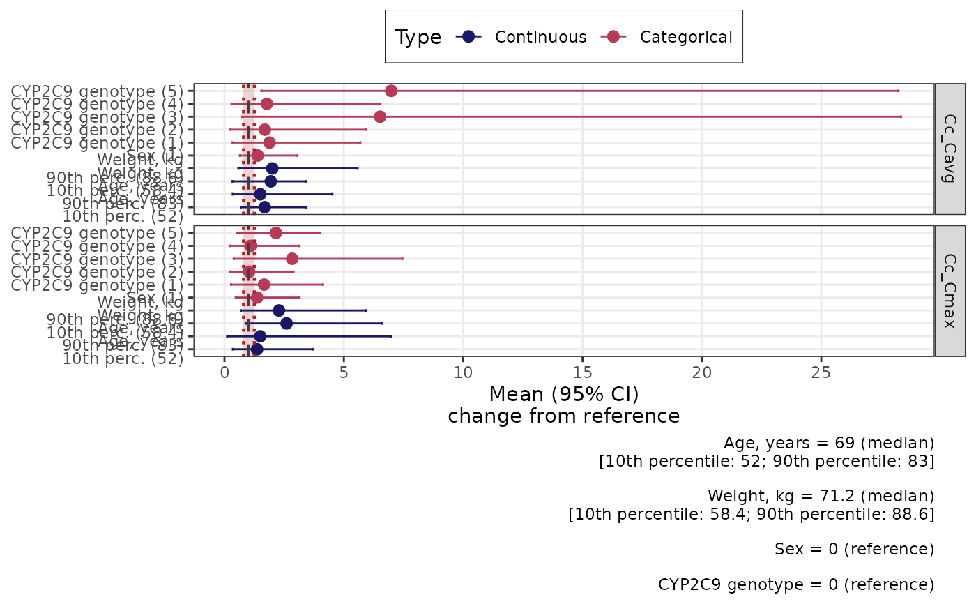
PARSENS— sensitivity of individual parameters (simulation at time zero, no ODE time course).EXPSENS— sensitivity of exposure summaries (e.g. Cmin, Cmax, Cavg) after full simulation overstimesinsg_covsens_sim.
Values on the y-axis are ratios relative to the reference scenario: 1
means no change. In sg_covsens_sim, percent change relative to
reference is transformed to this scale before tabulation. The shaded region
between ci_limits highlights a target interval; points whose
intervals lie largely inside can be read as scenarios consistent with that
criterion, subject to study-specific rules.
The plot layers are drawn in order: reference band, error bars, points,
reference line at 1, dotted lines at ci_limits, then faceting by
VAR and flipped coordinates so labels read along the vertical axis.
Examples
# \donttest{
library(tibble)
library(dplyr)
library(rxode2)
# Typical workflow: run the simulation (see examples in ?sg_covsens_sim),
# then visualise parameter and exposure sensitivity.
cont_cov_l <- list(
LG_AGE = list(NAME = "LG_AGE", UTNAME = "AGE",
REF = "median", NICENAME = "Age, years",
par_vec = c("CL")),
LG_WEIGHT = list(NAME = "LG_WEIGHT", UTNAME = "WEIGHT",
REF = "median", NICENAME = "Weight, kg",
par_vec = c("Vd"))
)
cat_cov_l <- list(
SEX = list(NAME = "SEX", NICENAME = "Sex",
REF = "0", par_vec = c("ka")),
CYP2C9 = list(NAME = "CYP2C9", NICENAME = "CYP2C9 genotype",
REF = NULL, par_vec = c("CL"))
)
# --- Dosing ---
ev_t_input <- tribble(
~id, ~time, ~ii, ~amt, ~addl, ~dur, ~evid, ~Regimen, ~Dose,
1, 0, 336, 10, 21, 0.5, 1, "0.3 mg/kg Q2W", 0.3
)
# --- Model ---
model <- RxODE({
# Doses in mg
# Time in hours
### Parameter values
# Typical values
ka_pop = 0.073;
Vd_pop = 14.8;
CL_pop = 0.347;
# Random effects
omega_ka = 0;
omega_Vd = 0;
omega_CL = 0;
# Covariate effect
# Continuous
beta_CL_LG_AGE = 0.49990114;
beta_Vd_LG_WEIGHT = 0.60529433;
# Categorical
beta_CL_CYP2C9_1_2 = -0.339;
beta_CL_CYP2C9_1_3 = -0.574;
beta_CL_CYP2C9_2_2 = -1.079;
beta_CL_CYP2C9_2_3 = -0.745;
beta_CL_CYP2C9_3_3 = -2.13;
beta_ka_SEX_1 = -0.12198035;
# Residual error
Cc_b = 0;
# Transformations
ka_tv = exp(ka_pop);
Vd_tv = exp(Vd_pop);
CL_tv = exp(CL_pop);
CL_multiplier = 1.0; # Default/reference
ka_multiplier = 1.0;
if (SEX == "1") {ka_multiplier = exp(beta_ka_SEX_1)}
if (CYP2C9 == "1") {
CL_multiplier = exp(beta_CL_CYP2C9_1_2);
} else if (CYP2C9 == "2") {
CL_multiplier = exp(beta_CL_CYP2C9_1_3);
} else if (CYP2C9 == "3") {
CL_multiplier = exp(beta_CL_CYP2C9_2_2);
} else if (CYP2C9 == "4") {
CL_multiplier = exp(beta_CL_CYP2C9_2_3);
} else if (CYP2C9 == "5") {
CL_multiplier = exp(beta_CL_CYP2C9_3_3);
}
ka = ka_tv*ka_multiplier*exp(omega_ka);
Vd = Vd_tv*exp(beta_Vd_LG_WEIGHT * LG_WEIGHT + omega_Vd); #Vd_tv*exp(omega_Vd);
CL = CL_tv*CL_multiplier*exp(beta_CL_LG_AGE * LG_AGE + omega_CL);
### Explicit functions
Cc = Ac/Vd;
### Initial conditions
Ad(0) = 0;
Ac(0) = 0;
### Differential equations
d/dt(Ad) = - ka*Ad;
d/dt(Ac) = ka*Ad - CL*Cc;
Cc_ResErr = Cc*(1 + Cc_b);
})
#>
#>
# --- Estimation covariance (mock) ---
pnames <- parest$parameter
npar <- length(pnames)
set.seed(1)
m_cov <- matrix(0.02, npar, npar)
diag(m_cov) <- 0.05 + runif(npar, 0, 0.05)
m_cov <- (m_cov + t(m_cov)) / 2
est_covmat <- as_tibble(cbind(X1 = pnames, as.data.frame(m_cov)))
names(est_covmat)[-1] <- pnames
# --- Simulation times (steady-state cycle 10) ---
ss_cycle <- 10
stimes_ss <- c(
ss_cycle * 4 * 7 * 24 + c(seq(0, 23.5, 0.5), seq(24, 335, 1)),
ss_cycle * 4 * 7 * 24 + 2 * 7 * 24 + c(seq(0, 23.5, 0.5), seq(24, 335, 1))
)
result <- sg_covsens_sim(
fpath_i = NULL, ds_parest = parest, ds_covs = ds_covval,
model = model, stimes = stimes_ss, et = ev_t_input,
est_covmat = est_covmat, npop = 10,
cont_cov_l = cont_cov_l, cat_cov_l = cat_cov_l,
quantiles = c(0.1, 0.9), aggr = c("min", "max", "mean"),
outputs = "Cc"
)
p_par <- sg_covsens_vis(result, plot_type = "PARSENS")
p_exp <- sg_covsens_vis(result, plot_type = "EXPSENS")
p_par
 p_exp
p_exp
 # Alternate interval columns (must exist in the sensitivity tables)
p <- sg_covsens_vis(result, ci = 95)
p
# Alternate interval columns (must exist in the sensitivity tables)
p <- sg_covsens_vis(result, ci = 95)
p
 # Drop selected metrics from the exposure panel
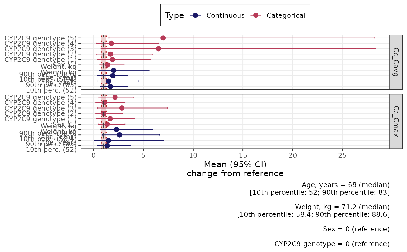
p <- sg_covsens_vis(result, plot_type = "EXPSENS", exclude_vars = c("Cc_Cmin"))
p
# Drop selected metrics from the exposure panel
p <- sg_covsens_vis(result, plot_type = "EXPSENS", exclude_vars = c("Cc_Cmin"))
p
 # }
# }