Installation
# Stable release
install.packages("SimuRg")

# Development version:
remotes::install_github("ms-decisions/SimuRg")
library(SimuRg)
#> Registered S3 method overwritten by 'sensitivity':
#>   method    from
#>   print.src dplyr
This package is designed for pharmacometricians and provides a
complete workflow for building, fitting, and evaluating population PK/PD
models. Model fitting, the first step of the workflow, is performed
using the sg_fit() function. Currently, two fitting engines
are supported: Monolix 2023 and Simurg cybernetic core. Both engines
must be installed separately, as they are not distributed with the
package. The fitting engine is selected using the opt_name argument.
Model calibration
To fit a model, several mandatory arguments must be provided. The
first is model, which specifies the path to the model file.
When using the Monolix fitting engine
(opt_name = "Monolix", the default), the model must be
written in the mlxtran format. When using the SimuRg Core engine
(opt_name = "Simurg"), both rxode2 and mlxtran model
formats are supported. In the following example, mlxtran format is
used.
library(tibble)
library(dplyr)
#>
#> Attaching package: 'dplyr'
#> The following objects are masked from 'package:stats':
#>
#>     filter, lag
#> The following objects are masked from 'package:base':
#>
#>     intersect, setdiff, setequal, union
library(stringr)
library(readr)

model <- system.file("extdata", "models", "model_PK_1c.txt", package = "SimuRg")
read_lines(model)
#>  [1] "DESCRIPTION:"
#>  [2] "The 1 comp. PK model with dose-dependent bioavailability."
#>  [3] ""
#>  [4] "[LONGITUDINAL]"
#>  [5] "input = {ka, V, Cl}"
#>  [6] ""
#>  [7] "PK:"
#>  [8] "; PK model definition"
#>  [9] "Cc = pkmodel(ka, V, Cl)"
#> [10] ""
#> [11] ";;; Priors"
#> [12] "MW = 627.57  \t\t\t\t\t; g/mol for INCB161734 "
#> [13] ""
#> [14] "OUTPUT:"
#> [15] "output = {Cc}"
Data specification
Next, the data argument must be used to specify the path
to the input dataset. The dataset should be provided in an ADPPK-like
format.
The structure of the dataset must be described using the headers argument, which is a list of column specifications. Each column specification is itself a list with the following elements:
-
name- character string specifying the name of the dataset column; -
use- character string defining the role of the column according to the Monolix data format specification (e.g.,"id","time","observation","covariate"); -
type- character string specifying the covariate type. For columns withuse = "covariate", this must be either “continuous” or “categorical”. For all other column types, this field should beNULL.
data  <- system.file("extdata", "datasets", "dspk-warf.csv", package = "SimuRg")
data_content <- read.csv(data)
head(data)
#> [1] "/home/runner/work/SimuRg/SimuRg/renv/library/linux-ubuntu-noble/R-4.6/x86_64-pc-linux-gnu/SimuRg/extdata/datasets/dspk-warf.csv"
headers <- list(list(name = "ID", use = "identifier", type = NULL),
                list(name = "TIME", use = "time", type = NULL),
                list(name = "DV", use = "observation", type = "continuous"),
                list(name = "DVID", use = "observationtype", type = NULL),
                list(name = "ADM", use = "administration", type = NULL),
                list(name = "AMT", use = "amount", type = NULL),
                list(name = "EVID", use = "eventidentifier", type = NULL),
                list(name = "MDV", use = "missingdependentvariable", type = NULL),
                list(name = "AGE", use = "covariate", type = "continuous"),
                list(name = "AGE_centered", use = "covariate", type = "continuous"),
                list(name = "SEX", use = "covariate", type = "categorical"),
                list(name = "WEIGHT", use = "covariate", type = "continuous"),
                list(name = "BMI", use = "covariate", type = "continuous"),
                list(name = "CLCR", use = "covariate", type = "continuous"),
                list(name = "CYP2C9_gentyp", use = "covariate", type = "categorical"),
                list(name = "VKORC1_gentyp", use = "covariate", type = "categorical"),
                list(name = "G1_1", use = "ignore", type = NULL),
                list(name = "G1_2", use = "ignore", type = NULL),
                list(name = "G1_3", use = "ignore", type = NULL),
                list(name = "G2_2", use = "ignore", type = NULL),
                list(name = "G2_3", use = "ignore", type = NULL),
                list(name = "G3_3", use = "ignore", type = NULL),
                list(name = "GG", use = "ignore", type = NULL),
                list(name = "AG", use = "ignore", type = NULL),
                list(name = "AA", use = "ignore", type = NULL))
Statistical components
After specifying the model and dataset, the statistical components of
the model must be defined. The first is the theta argument,
which is a data frame describing the model parameters and their
estimation settings. It must contain the following columns:
-
NAME– character string specifying the parameter name; -
TRANS– character string specifying the parameter distribution. Supported values are"normal","logNormal", and"logitNormal"; -
INIT– numeric value specifying the initial estimate or, for fixed parameters, the fixed value; -
LB– numeric value specifying the lower bound for parameters with a"logitNormal"distribution. For all other distributions, this value should beNA; -
UB– numeric value specifying the upper bound for parameters with a"logitNormal"distribution. For all other distributions, this value should beNA. -
EST– logical value indicating whether the parameter should be estimated (TRUE) or fixed (FALSE).
In our example, all parameters will be estimated and will have the lognormal distribution
theta <- tribble(~NAME, ~TRANS, ~INIT, ~LB, ~UB, ~EST,
                  "Cl", "logNormal", 0.2, NA, NA, TRUE,
                  "V", "logNormal", 20, NA, NA, TRUE,
                  "ka", "logNormal", 0.2, NA, NA, TRUE
)
The second statistical component defines the random effects and is
specified using the re argument. This object consists of
two square matrices with dimensions equal to the number of model
parameters:
init– specifies the initial values of the random-effects covariance matrix.-
est– specifies how each element of the covariance matrix is treated during estimation:-
TRUE– the corresponding element is estimated. -
FALSE– the corresponding element is fixed at its initial value. -
NA– the corresponding random effect is omitted from the model.
-
The rows and columns of both matrices correspond to the model
parameters defined in the theta data frame.
Between-occasion variability, defined by occ parameter,
is specified in the same way, as the re parameter.
In our case, we will add the between subjects variability to
Cl and ka parameters. No between-occasion
variability will be added.
re <- list(init = tribble(~Cl, ~V, ~ka,
                           1, 0, 0,
                           0, 0, 0,
                           0, 0, 1) %>% as.matrix(),
            est = tribble(~Cl, ~V, ~ka,
                          TRUE, NA, NA,
                          NA, NA, NA,
                          NA, NA, TRUE) %>% as.matrix())

occ <- list(init = tribble(~Cl, ~V, ~ka,
                            0, 0, 0,
                            0, 0, 0,
                            0, 0, 0) %>% as.matrix(),
             est = tribble(~Cl, ~V, ~ka,
                           NA, NA, NA,
                           NA, NA, NA,
                           NA, NA, NA) %>% as.matrix())
The last statistical component specifies the residual unexplained variability (RUV) model and is provided through the ruv argument. This object is a list of observation-specific specifications, where each element is itself a list with the following fields:
-
YNAME– character string specifying the observation name (typically “y1”, “y2”, etc.); -
DVID– numeric identifier of the observation type, corresponding to the values in the DVID column of the dataset; -
TRANS– character string specifying the residual error distribution. Supported values are “normal”, “logNormal”, and “logitNormal”; -
PRED– character string specifying the name of the prediction variable defined in the model; -
ERR– character string specifying the residual error model. Supported values are “constant” (additive error), “proportional” (proportional error), and “combined1” (combined additive and proportional error); -
INIT– numeric vector containing the initial values of the residual error parameters. The required length depends on the selected error model; -
EST– logical vector indicating whether each residual error parameter should be estimated (TRUE) or fixed (FALSE). This vector must have the same length as INIT; -
BLQM– below-limit-of-quantification (BLQ) handling method. If no BLQ method is used, this field should be NULL.
In our example, we have one DVID, therefore ruv object will have the following structure:
Covariates
Finally, covariate effects can be specified using the
cov argument. This argument is a list of covariate
specifications, where each element is itself a list with the following
fields:
-
PAR– character string specifying the name of the model parameter to which the covariate effect is applied. -
COVNAME– character string specifying the name of the covariate. -
FUNC– character string specifying the functional form of the covariate effect. Supported values are"linear"for continuous covariates and"categorical"for categorical covariates. -
TRANS– character string specifying the covariate transformation. Supported values are"median"for continuous covariates and"reference"for categorical covariates. -
INIT– numeric value specifying the initial estimate of the covariate effect. -
EST– logical value indicating whether the covariate effect should be estimated (TRUE) or fixed (FALSE).
Model calibration
The sg_fit() function also provides several optional
arguments:
-
project_name– character string specifying the project name. This name is used for the generated.mlxtranfile and the output directory containing the fitting results. -
fit– logical value indicating whether model fitting should be performed. IfFALSE, only the control object (either a.mlxtranproject or aGCOobject, depending on the selected engine) is generated. -
path_to_save_output– path to the directory where the output files will be saved. -
path_to_fitter– path to the fitting engine executable. -
max_wait_time– maximum time (in seconds) to wait for the fitting process to complete.
The model can now be fitted by calling sg_fit(). Since
neither Monolix nor Simurg core is available in the environment used to
build this vignette, the fitting step is skipped by setting
fit = FALSE. In this case, only the control object is
generated. The resulting control object can subsequently be submitted to
the corresponding fitting engine in a separate environment where the
required software is installed.
output_path <- str_c(tempdir(), "/")
task_opt <-  paste("populationParameters()", "individualParameters()",
                    "logLikelihood()", sep = "\n")
result <- sg_fit(model, data, headers, theta, ruv, re, occ, covs,
                  project_name = "my_project", fit = FALSE, # set fit = TRUE for fit
                  path_to_save_output =  output_path)
#> The file for fit was written /tmp/RtmpuAXqXL/my_project.mlxtran
Reading model calibration results
Another option of SimuRg package is not to fit a model inside the
package, but just read Monolix/Simurg fit results. For this goal,
sg_converter() function can be used. Its use and
specification is simpler, than the use of sg_fit(), as it
has only three arguments:
- folder_path - character string with path to the directory with Monolix project files
- proj_name - character string with the name of the project
test_folder <- system.file("extdata", "Monolix_objects", package = "SimuRg")
if (substr(test_folder, nchar(test_folder), nchar(test_folder)) != "/")
  test_folder <- str_c(test_folder, "/")
pro_name <- "proj-solo"
message("Resolved folder: ", test_folder)
#> Resolved folder: /home/runner/work/SimuRg/SimuRg/renv/library/linux-ubuntu-noble/R-4.6/x86_64-pc-linux-gnu/SimuRg/extdata/Monolix_objects/
message("Folder exists: ", dir.exists(test_folder))
#> Folder exists: TRUE

result <- sg_converter(folder_path = test_folder, proj_name = pro_name)
#> Detected model structure:1comp_ka
#> Omega parameters: omega_ka, omega_Cl
#> Random effect parameters:ka, Cl
#> Using Monte Carlo simulation with n_sim = 1000
#> Extracted parameter distributions: 3 parameters
#>   %s: %s (typical=%.2f, sd=%.2f)
#> CllogNormalCl_popomega_Cl
#>   %s: %s (typical=%.2f, sd=%.2f)
#> VlogNormalV_popNA
#>   %s: %s (typical=%.2f, sd=%.2f)
#> kalogNormalka_popomega_ka
#> Joining with `by = join_by(id)`
sg_converter() and sg_fit() objects return
GCO and GFO objects, which are inputs for
other functions of the package. Please check the documentation to see
the.
Goodness-of-fit
Basic GoF plots
Now, when the model was calibrated, one can do model diagnostics.
SimuRg package include following functions for model goodness of fit
diagnostics: * sg_gof_obpr() - observed versus predicted
plot; * sg_gof_tp() - time profiles visualization; *
sg_gof_par_cov() - visualization of random
effect/individual parameters vs covariated; *
sg_gof_par_dist() - plot the distribution of random
effects/individual parameters; * sg_gof_res_dist() - plot
the distribution of the residual * sg_gof_res() - create
residual diagnostic plots
sg_gof_obpr(result$GFO)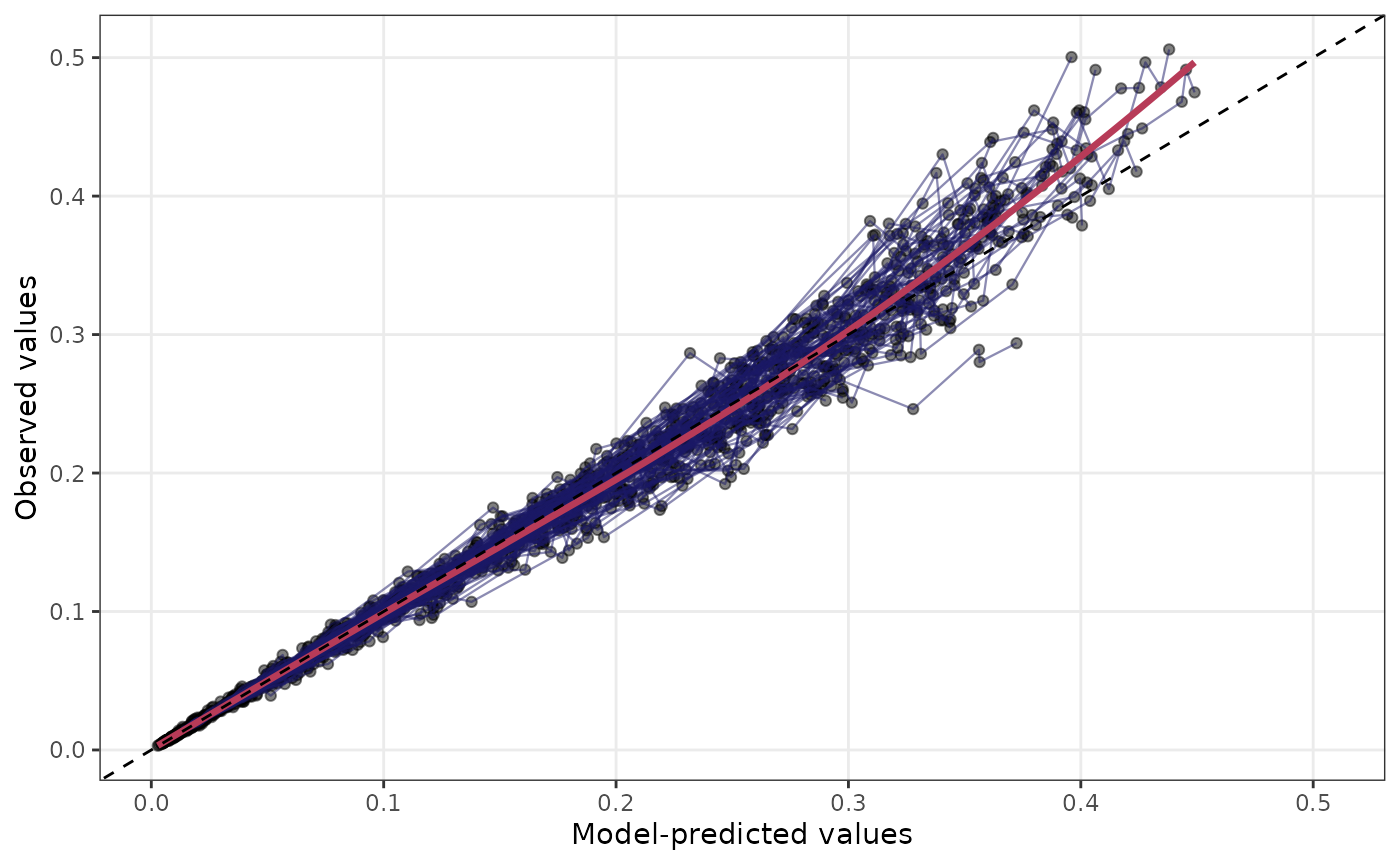
sg_gof_tp(result$GFO)
#> [[1]]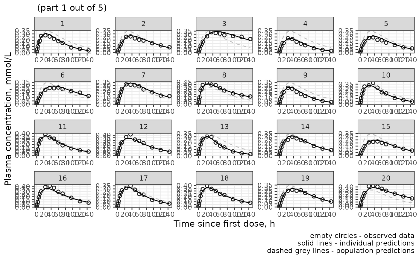
#>
#> [[2]]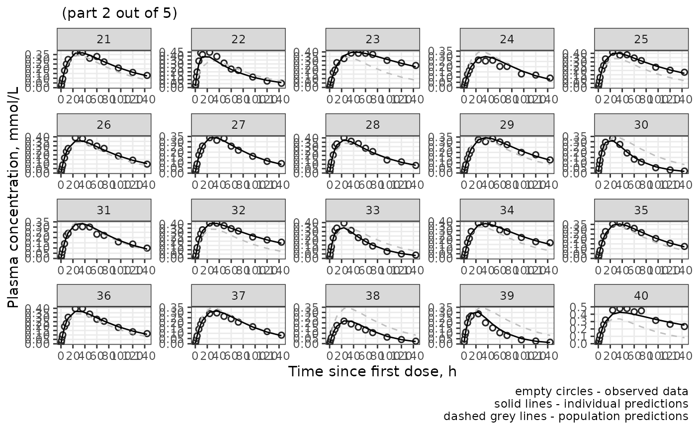
#>
#> [[3]]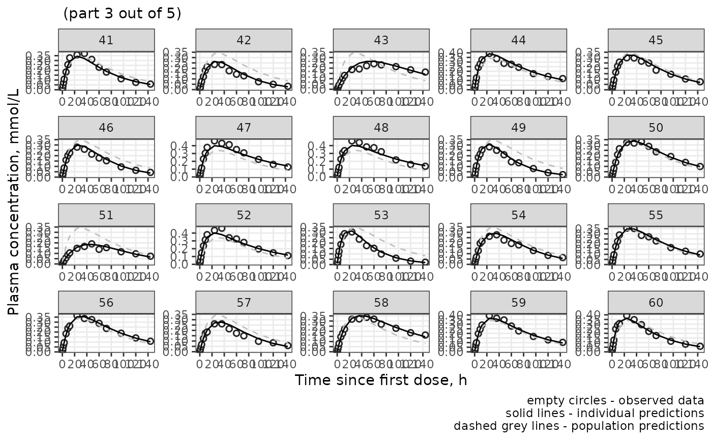
#>
#> [[4]]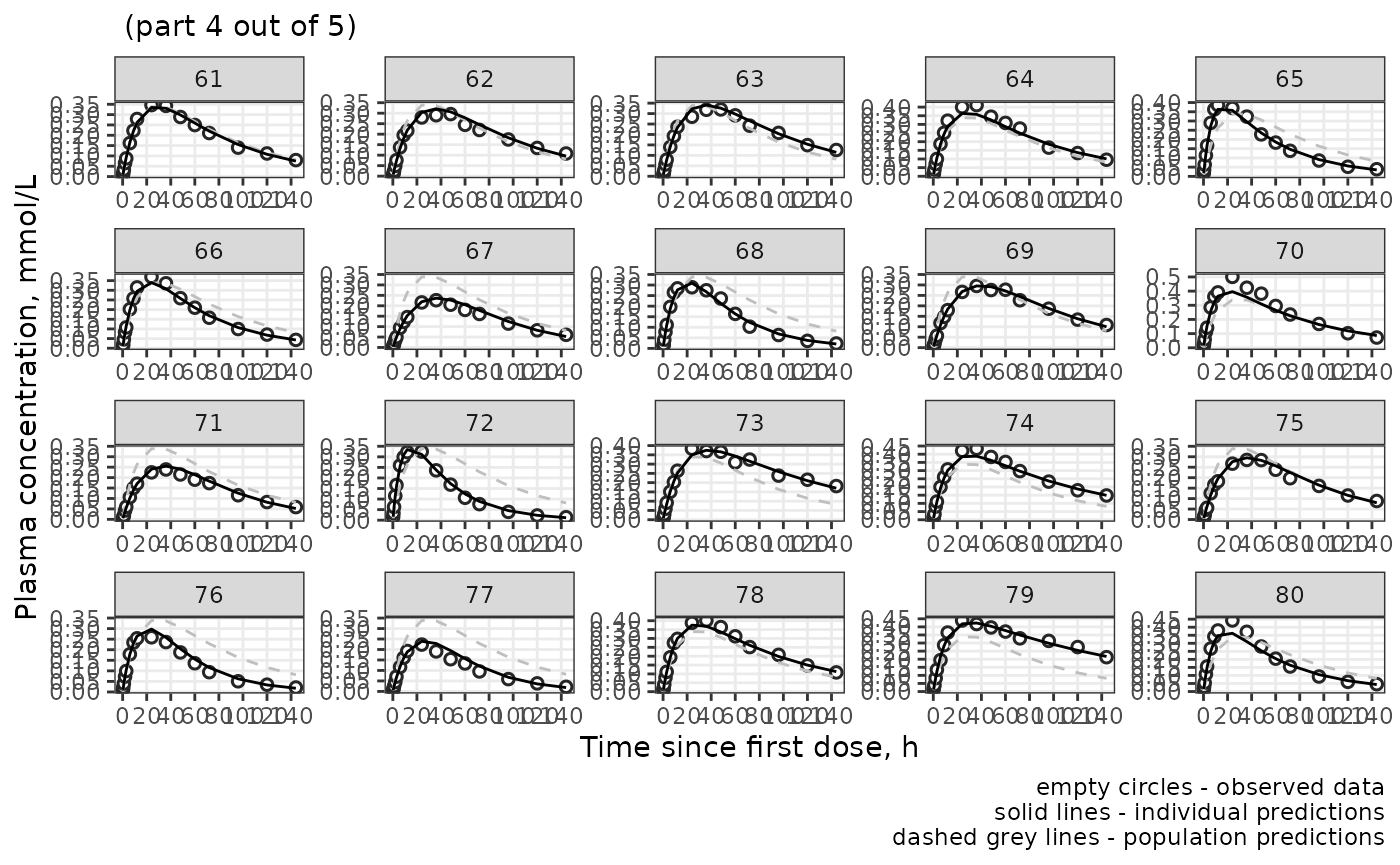
#>
#> [[5]]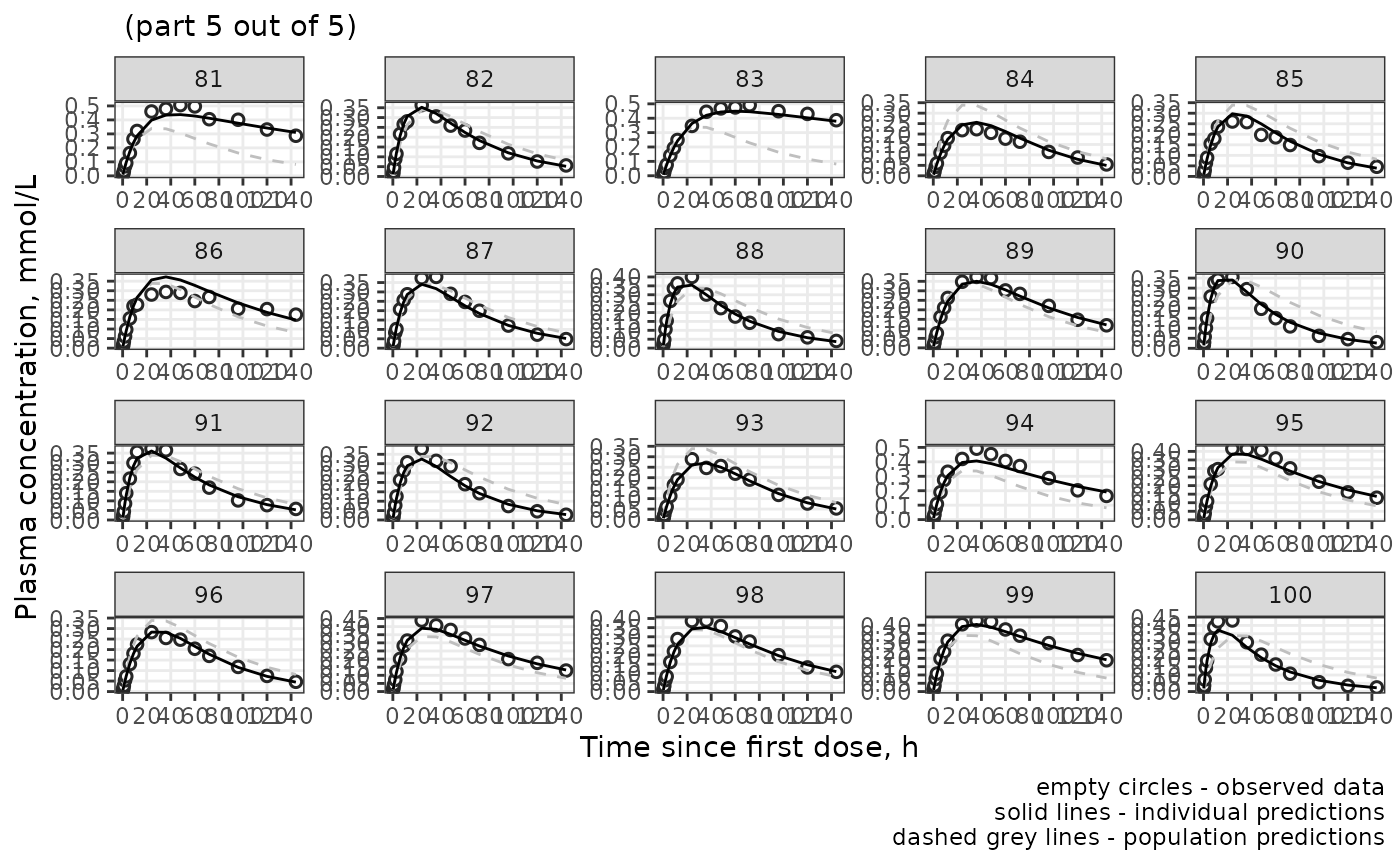
sg_gof_par_dist(result$GFO)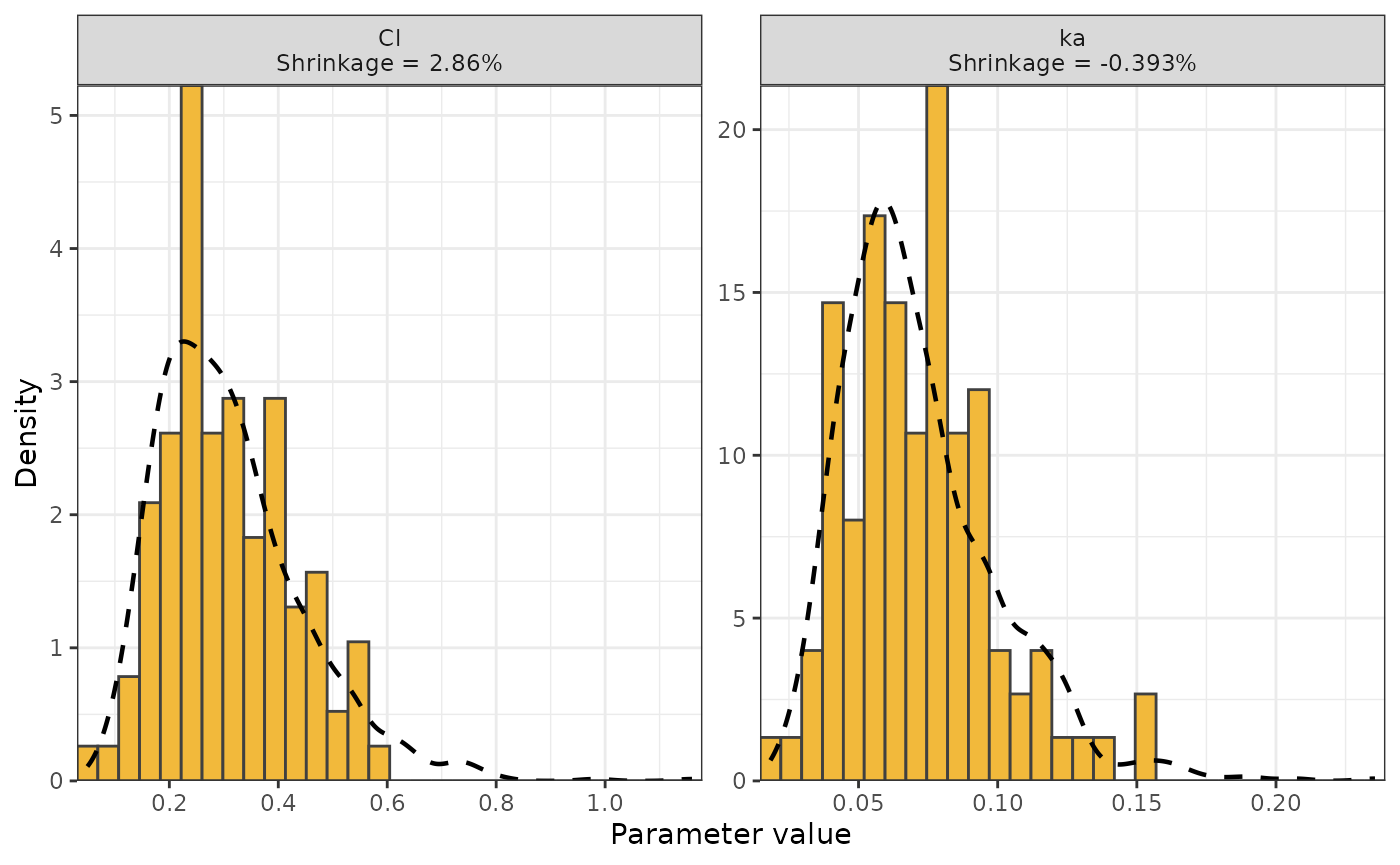
sg_gof_res_dist(result$GFO)
#> Warning: The dot-dot notation (`..density..`) was deprecated in ggplot2 3.4.0.
#> ℹ Please use `after_stat(density)` instead.
#> ℹ The deprecated feature was likely used in the SimuRg package.
#>   Please report the issue at <https://github.com/ms-decisions/SimuRg/issues>.
#> This warning is displayed once per session.
#> Call `lifecycle::last_lifecycle_warnings()` to see where this warning was
#> generated.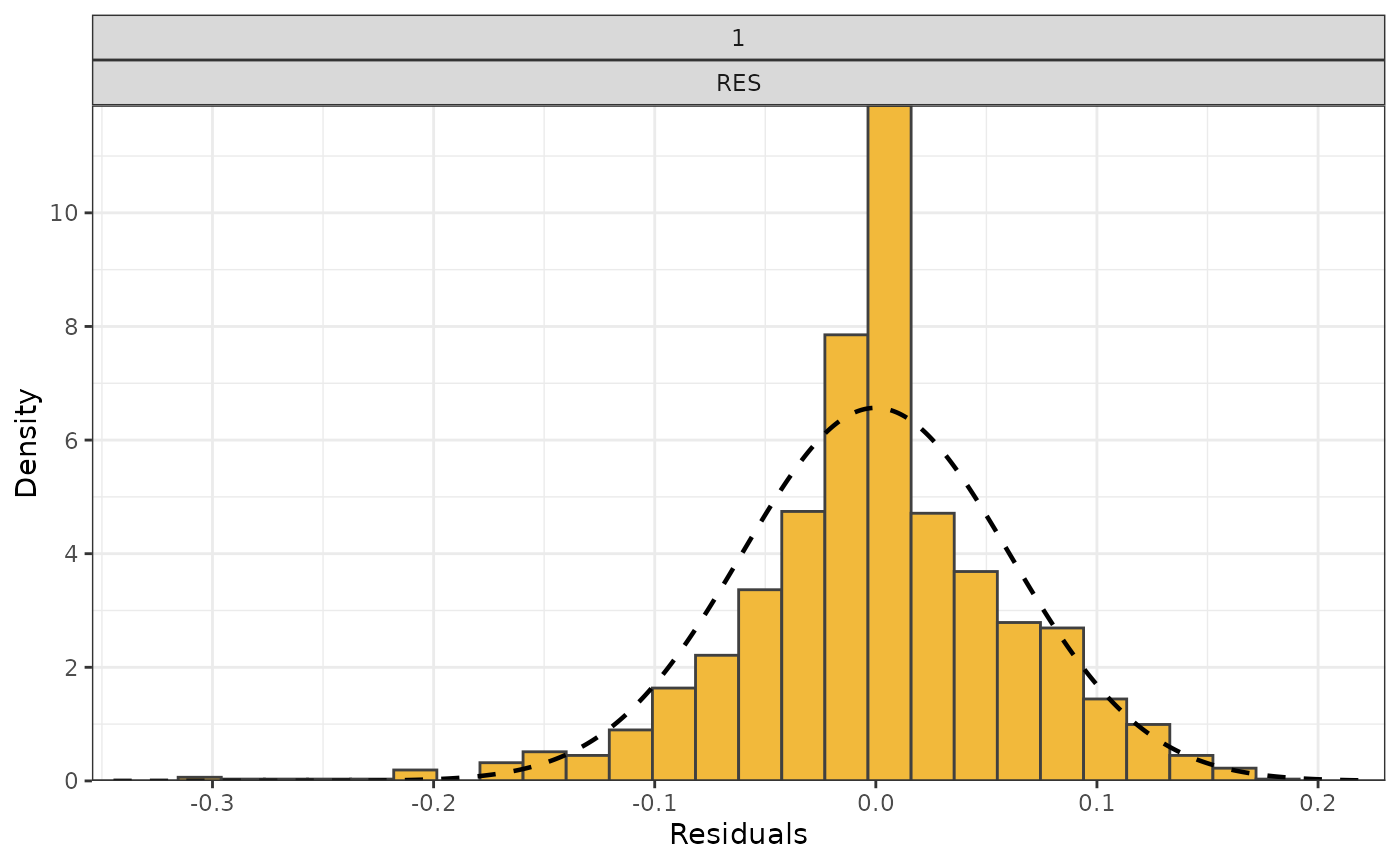
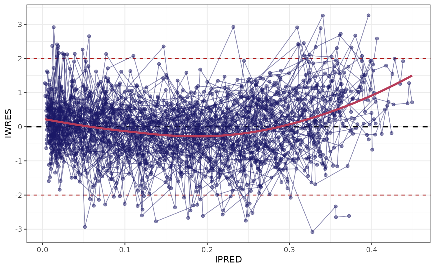
sg_gof_res(result$GFO)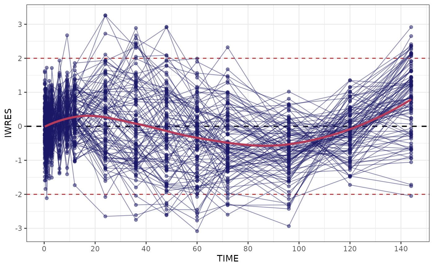
sg_gof_res(result$GFO, vs_time = F)