Observed vs predicted plot

Function generates observed versus predicted scatter plots from GFO $SDTAB, a fundamental goodness-of-fit diagnostic tool in pharmacometric modeling. This visualization assesses model adequacy by comparing observed clinical measurements against model-predicted values, enabling identification of systematic bias, heteroscedasticity, and model misspecification patterns. Function contains options for faceting, coloring by covariates, and trend lines.

Usage

sg_gof_obpr(
  fpath_i,
  DVID = 1,
  cov_cols = NULL,
  indiv = TRUE,
  addline = TRUE,
  alpha_i = 0.5,
  smooth = TRUE,
  log_axes = FALSE,
  sc_factor = 1,
  abreaks = scales::pretty_breaks(7),
  lab_x = "Model-predicted values",
  lab_y = "Observed values",
  col_i = NULL,
  col_lab = NULL,
  facet_i = NULL,
  f_scales = "fixed",
  no_leg = FALSE,
  n_quantiles = 3,
  levels_discrete = 10
)

Arguments

fpath_i

String, GFO, or a named list with a GFO component (and optionally GCO). If a string is given, the path to a .RData or .json file with a fit object is expected.

DVID

Restrict SDTAB to one observation type. Numeric values select the DVID column (default 1). If SDTAB has DVNAME, a character or factor is matched to DVNAME first; otherwise a digit-only string is coerced to numeric DVID.

cov_cols

A character vector specifying the names of the columns with covariates.

indiv

Logical. If TRUE, use individual predictions ("IPRED"); otherwise use population predictions ("PRED"). Default is TRUE.

addline

Logical. If TRUE, lines connecting observations of individual subjects will be added. Default is TRUE.

alpha_i

Numeric. Transparency level (from 0 to 1) for points/lines. Default is 0.5.

smooth

Logical. Add LOESS smooth line. Default is TRUE.

log_axes

Logical. If TRUE, a logarithmic scale is applied to all axes. Default is FALSE.

sc_factor

Numeric. Scaling factor for DV/PRED/IPRED values. Default is 1 (no scaling).

abreaks

A function that generates axis breaks. Default is scales::pretty_breaks(7).

lab_x

X-axis label. Default "Model-predicted values"

lab_y

Y-axis label. Default "Observed values"

col_i

String. Column name for color

col_lab

String. Label for color legend

facet_i

Character vector. Column name(s) for facet panels. Multiple columns are combined with + in facet_wrap. Default is NULL.

f_scales

String, one of "fixed", "free", "free_x", "free_y". User can specify whether the scales (x and y axes) should be fixed across all panels ("fixed"), free for each panel ("free"), or free only in one dimension ("free_x" or "free_y"). Default is "fixed"

no_leg

Logical. If TRUE, the legend is not shown. Default is FALSE

n_quantiles

Integer. Number of quantile groups for continuous variables in col_i. Default is 3.

levels_discrete

Integer. Maximum unique values to consider a variable discrete. Default is 10.

Value

A ggplot2 object

Examples

# \donttest{
# Basic example with mock data
set.seed(123)  # For reproducibility
mock_obj <- list(
 SDTAB = data.frame(
   ID = rep(1:3, each = 5),
   TIME = rep(c(0, 1, 2, 4, 8), 3),
   DV = rnorm(15, mean = 10, sd = 2),
   PRED = rnorm(15, mean = 10, sd = 1.5),
   IPRED = rnorm(15, mean = 10, sd = 1.2),
   MDV = rep(0, 15)
 ),
 COTAB = data.frame(ID = 1:3, AGE = c(30, 45, 60)),
 CATAB = data.frame(ID = 1:3, RACE = c("Hispanic", "Hispanic", "Asian"))
)

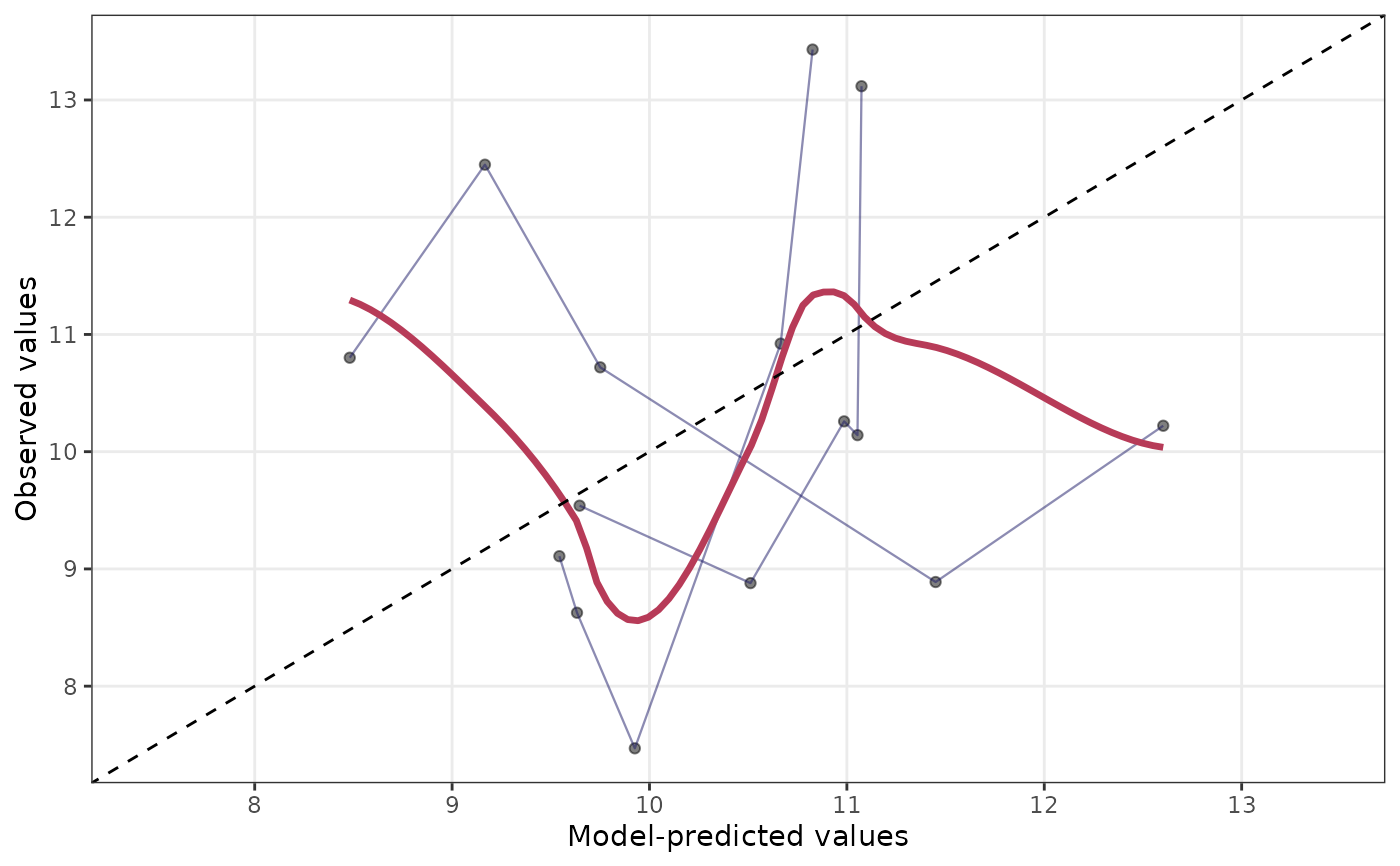
# Basic plot
p <- sg_gof_obpr(mock_obj)
p


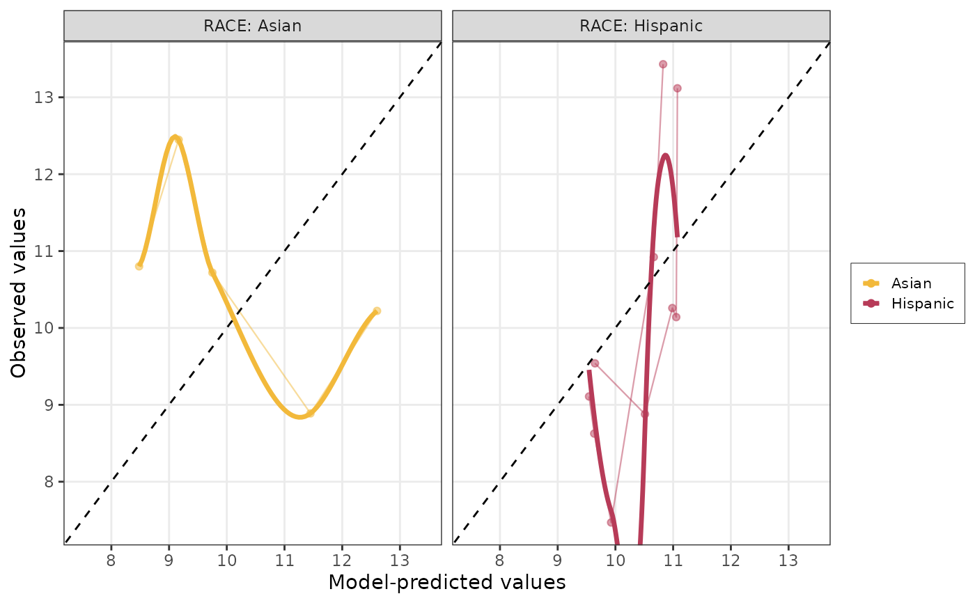
# With covariates and faceting
p <- sg_gof_obpr(
  mock_obj,
  cov_cols = "RACE",
  col_i = "RACE",
  facet_i = "RACE"
)
p
#> Warning: span too small.   fewer data values than degrees of freedom.
#> Warning: pseudoinverse used at 8.4609
#> Warning: neighborhood radius 1.2896
#> Warning: reciprocal condition number  0
#> Warning: There are other near singularities as well. 8.2533
#> Warning: Chernobyl! trL>n 5
#> Warning: Chernobyl! trL>n 5
#> Warning: NaNs produced

# }