
Plot distributions of individual parameters with optional theoretical density
Source:R/sg-gof-par-dist.R
sg_gof_par_dist.RdThis function creates histograms of individual parameter estimates, with optional overlay of the theoretical distribution based on the population parameters and OMEGA matrix.
Usage
sg_gof_par_dist(
  fpath_i,
  par_seq = NULL,
  par_type = "Ind",
  n_bins = 30,
  tdist = TRUE,
  plot_type = "DIST"
)
Arguments
- fpath_i
String, GFO, or a named list with a
GFOcomponent (and optionallyGCO). If a string is given, the path to a.RDataor.jsonfile with a fit object is expected.- par_seq
Vector of strings. Character vector of parameter names to be plotted. If
NULL, all parameters be included. Default isNULL- par_type
String. A character string specifying the type of parameters used for theoretical distribution overlay (only relevant when
plot_type = 'DIST'andtdist = TRUE). If 'Ind' - Individual (default), distributions are shown on the natural parameter scale assuming log-normal variability. If 'RE' - Random Effect, distributions are shown on the ETA scale, assuming a normal distribution with mean zero and covariance defined by$OMEGAMAT, without transformation.- n_bins
Integer. Number of bins to use in the histogram. Default is 30.
- tdist
Logical. If
TRUE, overlay theoretical parameter distributions based on population mean and OMEGA matrix. Default isTRUE.- plot_type
Character string specifying the type of plot to generate. Options: 'DIST' for parameter distributions (default), 'QQ' for Q-Q plots, 'correlations' for correlation matrix plot.
Value
A ggplot object containing histogram(s) of individual parameter distributions, optionally overlaid with theoretical densities.
Details
The function visualizes the distribution of post hoc individual parameter estimates
(from GFO $PATAB) and optionally compares them with the expected population-level
variability using $SUMTAB$DISTRIBUTION (see Details).
Shrinkage values are calculated based on ETAshrinkage_var from $SUMTAB and included in facet labels.
Theoretical distributions are generated by sampling from a multivariate normal distribution (mean zero, covariance from $OMEGAMAT) and mapping to the individual-parameter scale using typical values and the DISTRIBUTION column: logNormal uses TV * exp(ETA), normal uses TV + ETA, logitNormal uses the inverse logit of logit(TV) + ETA. Parameters with missing or empty DISTRIBUTION do not get a theoretical curve.
Examples
# \donttest{
# Basic usage: distribution plots for all parameters
fpath_i <- system.file("extdata", "simurg_object", "Warfarin_PK.RData", package = "SimuRg")
p <- sg_gof_par_dist(fpath_i = fpath_i)
p
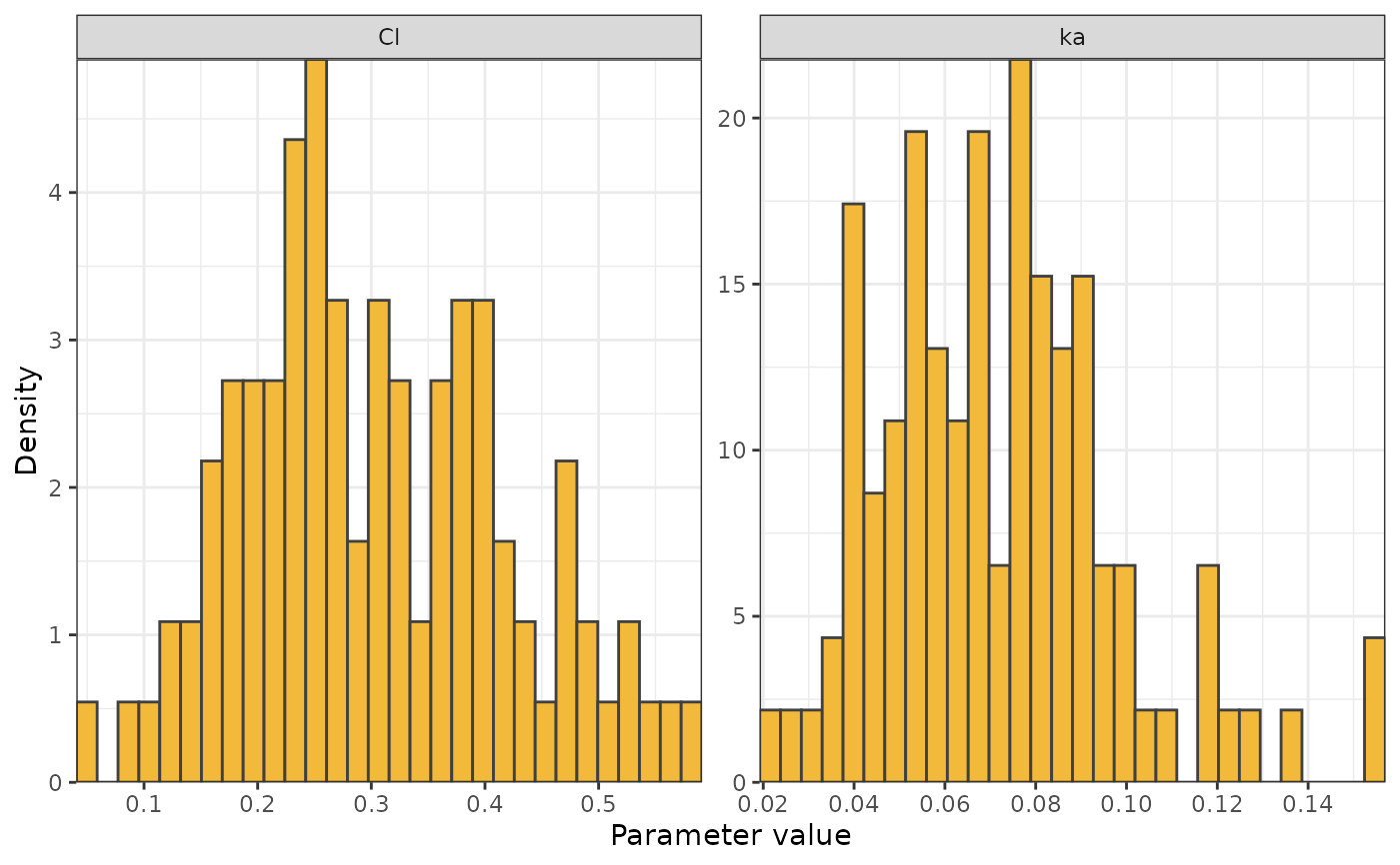 # Distribution plots for selected parameters (natural scale)
p <- sg_gof_par_dist(fpath_i = fpath_i, par_seq = c("ka", "Cl"))
p
# Distribution plots for selected parameters (natural scale)
p <- sg_gof_par_dist(fpath_i = fpath_i, par_seq = c("ka", "Cl"))
p
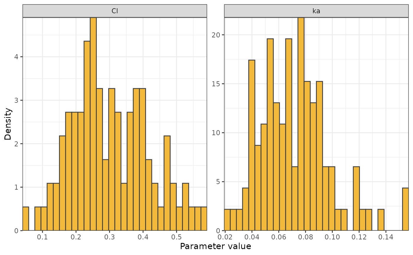
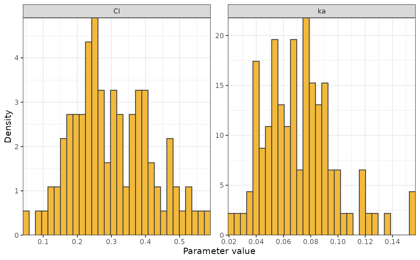 # Distribution plots with theoretical densities disabled
p <- sg_gof_par_dist(fpath_i = fpath_i, tdist = FALSE)
p
# Distribution plots with theoretical densities disabled
p <- sg_gof_par_dist(fpath_i = fpath_i, tdist = FALSE)
p
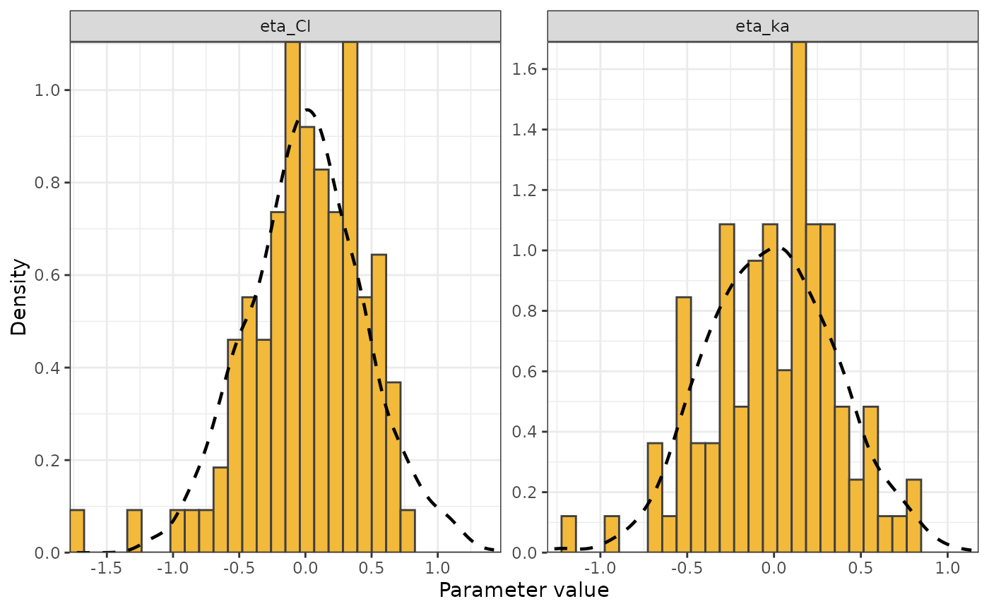
 # Distribution plots for ETA
p <- sg_gof_par_dist(fpath_i = fpath_i, par_seq = c("eta_ka", "eta_Cl"), par_type = "RE")
p
# Distribution plots for ETA
p <- sg_gof_par_dist(fpath_i = fpath_i, par_seq = c("eta_ka", "eta_Cl"), par_type = "RE")
p
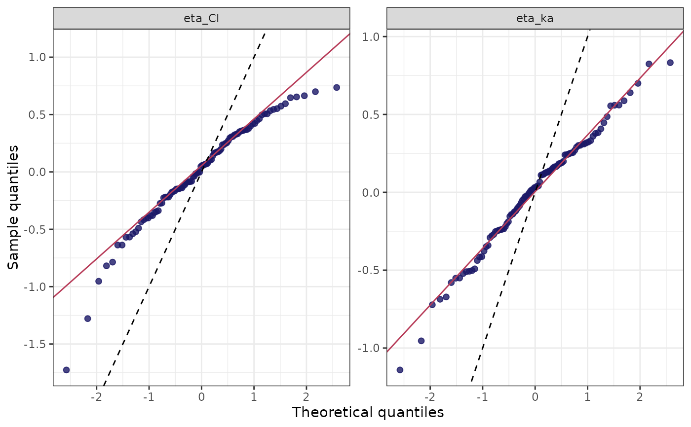
 # Q-Q plots for all ETA parameters
p <- sg_gof_par_dist(fpath_i = fpath_i, plot_type = "QQ")
p
# Q-Q plots for all ETA parameters
p <- sg_gof_par_dist(fpath_i = fpath_i, plot_type = "QQ")
p
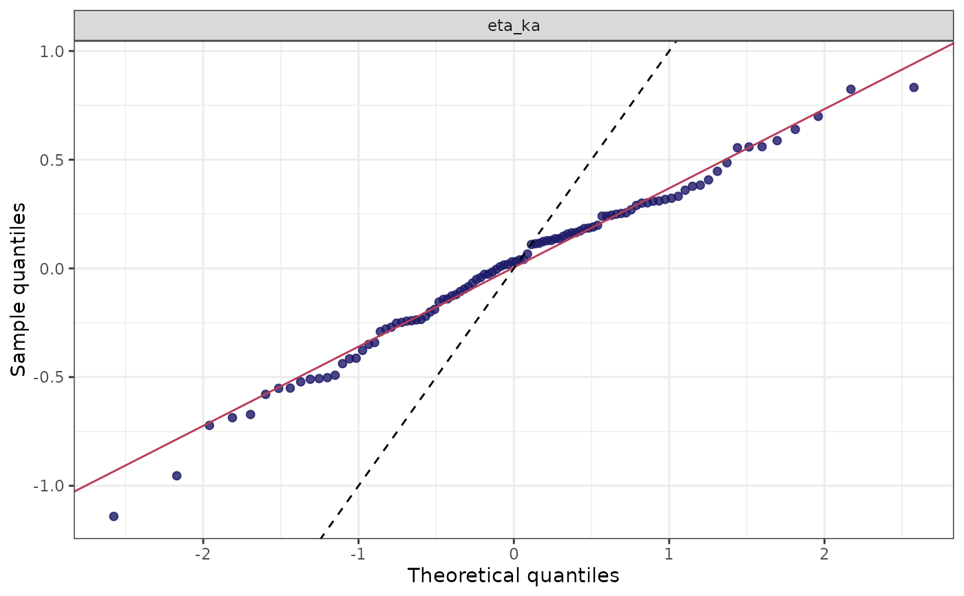
 # Q-Q plot for a specific ETA parameter
p <- sg_gof_par_dist(fpath_i = fpath_i, plot_type = "QQ", par_seq = "eta_ka")
p
# Q-Q plot for a specific ETA parameter
p <- sg_gof_par_dist(fpath_i = fpath_i, plot_type = "QQ", par_seq = "eta_ka")
p
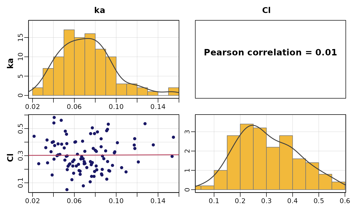
 # Correlation matrix for selected parameters
p <- sg_gof_par_dist(fpath_i = fpath_i, plot_type = "correlations")
# Correlation matrix for selected parameters
p <- sg_gof_par_dist(fpath_i = fpath_i, plot_type = "correlations")
 p
p
 # }
# }