Visualize Local Sensitivity Analysis Results

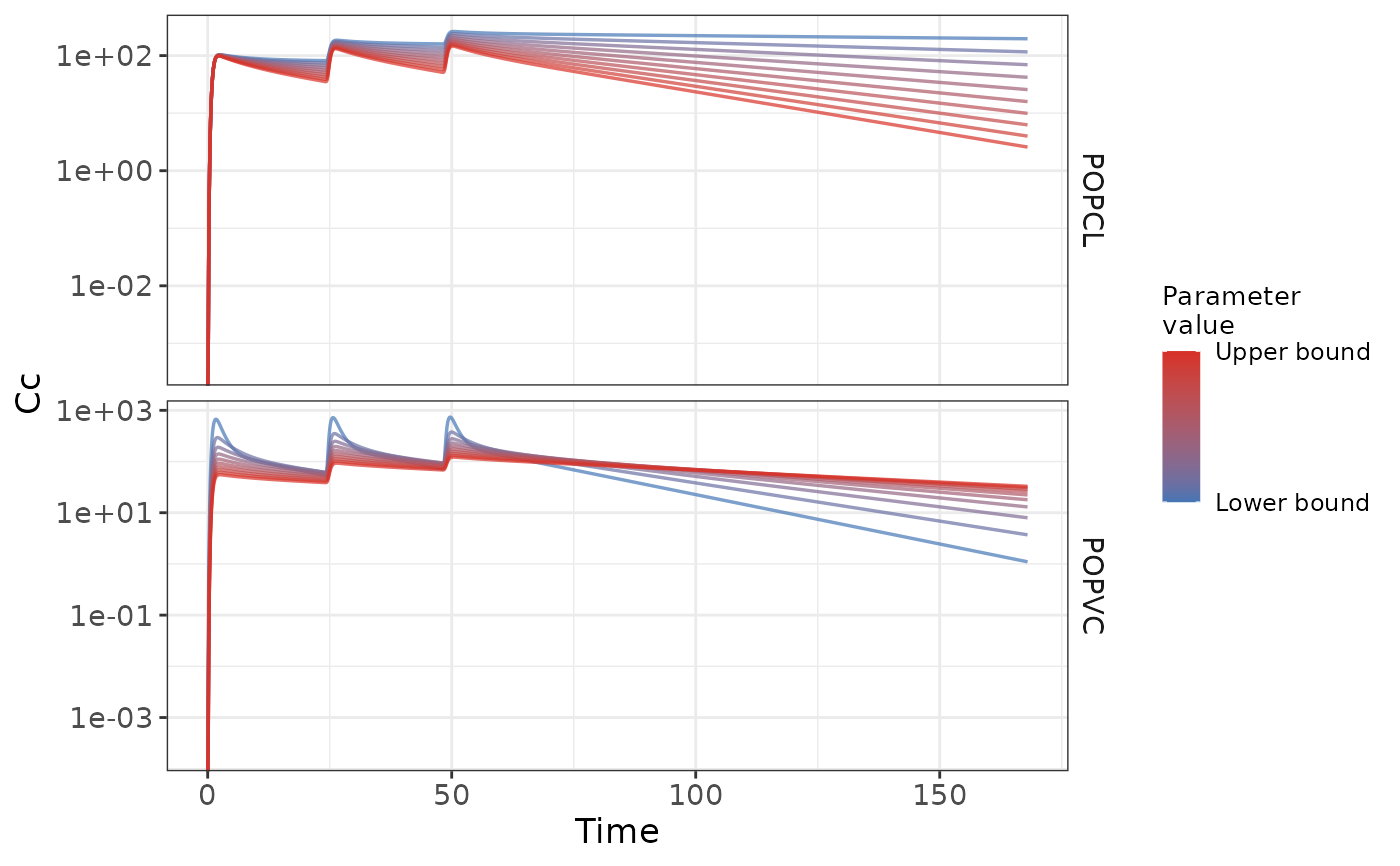
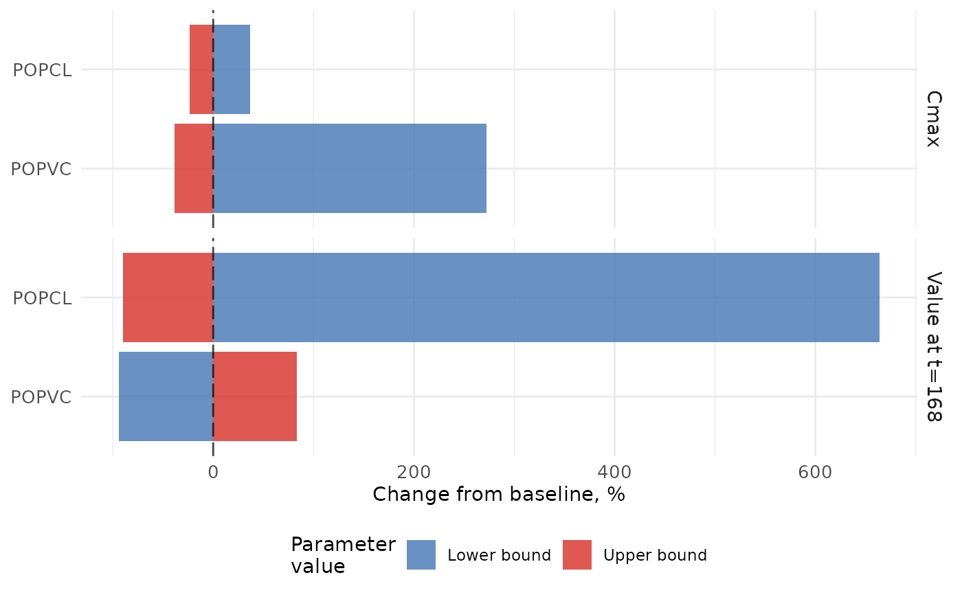
This function creates plots to visualize the results of a local sensitivity analysis: (1) a family of curves plot showing how model outputs vary over time for different parameter perturbations, and (2) a tornado plot summarizing the relative influence of each parameter on selected summary metrics (e.g., output value at a chosen time or Cmax).

Usage

sg_localsens_vis(
  sens_data,
  tornado_time = NULL,
  metrics = "value",
  ref_data = NULL,
  log_scale = FALSE,
  color_low = "#1f77b4",
  color_high = "#ff7f0e",
  facet_scales = "free"
)

Arguments

sens_data

A data frame containing sensitivity analysis results from sg_localsens_sim()

tornado_time

Numeric value specifying the time point (in the same units as TIME) at which to evaluate the model output for the tornado plot. Defaults to the maximum time in sens_data if not specified.

metrics

Character vector specifying which metrics to include in the tornado plot. Supported options are "value" (value at tornado_time) and "cmax" (maximum output). Defaults to "value".

ref_data

Optional data frame providing reference (baseline) output values, formatted similarly to sens_data. If NULL, the function uses the mid-range parameter value as the baseline.

log_scale

Logical. If TRUE, the y-axis of the family-of-curves plot is displayed on a log scale.

color_low

Character. Color used for the lower parameter bound (default: "#1f77b4").

color_high

Character. Color used for the upper parameter bound (default: "#ff7f0e").

facet_scales

Character string passed to facet_grid(), defining how y-axis scales behave across facets (default = "free").

Value

A named list containing:

family_of_curves

A ggplot2 object showing parameter sensitivity curves over time.

tornado

A ggplot2 object showing the tornado plot of relative sensitivity.

Examples

# \donttest{
library(rxode2)
library(tibble)
mod_ex <- RxODE({
  # Doses in mg
  # Time in hours
  ### Parameter values
  # Typical
  POPCL = 5;
  POPVC = 180;
  POPQ = 7;
  POPVP = 52;
  POPKTR = 6;
  FBIOPAR = 1;
  # Covariate coefficients
  POPIGFRCOV = 0.8;
  POPPATCOVCLGR1 = 0.85;
  POPPATCOVCLGR2 = 0.85;
  POPPATCOVCLGR3 = 0.85;
  POPPATCOVCLGR4 = 0.85;
  # Random effects
  PPVCL = 0;
  PPVVC = 0;
  PPVKTR = 0;
  # Residual error
  RUV = 0;
  ### Covariates
  PATCOVCL = 1
  if(POPN == 1){PATCOVCL = POPPATCOVCLGR1}
  if(POPN == 2){PATCOVCL = POPPATCOVCLGR2}
  if(POPN == 3){PATCOVCL = POPPATCOVCLGR3}
  if(POPN == 4){PATCOVCL = POPPATCOVCLGR4}
  IGFRCOV = (IGFR/112)^POPIGFRCOV
  ## Parameters
  CL = POPCL * IGFRCOV * PATCOVCL * exp(PPVCL);
  VC = POPVC * exp(PPVVC);
  Q = POPQ;
  VP = POPVP;
  KTR = POPKTR * exp(PPVKTR);
  ### Explicit functions
  Cc = Ac/VC;                 # nmol/L
  Cp = Ap/VP;                 # nmol/L
  ### Initial conditions
  At1(0) = 0;         # mg
  At2(0) = 0;         # mg
  At3(0) = 0;         # mg
  At4(0) = 0;         # mg
  At5(0) = 0;         # mg
  At6(0) = 0;         # mg
  Ad(0) = 0;          # mg
  Ac(0) = 0;          # mg
  Ap(0) = 0;          # mg
  ### ODEs
  d/dt(At1) = - KTR*At1;
  d/dt(At2) = KTR*At1 - KTR*At2;
  d/dt(At3) = KTR*At2 - KTR*At3;
  d/dt(At4) = KTR*At3 - KTR*At4;
  d/dt(At5) = KTR*At4 - KTR*At5;
  d/dt(At6) = KTR*At5 - KTR*At6;
  d/dt(Ad) = KTR*At6 - KTR*Ad;
  d/dt(Ac) = KTR*Ad - CL*Cc - Q*(Cc - Cp);
  d/dt(Ap) = Q*(Cc - Cp);
  FBIO = FBIOPAR
  f(At1) = FBIO*1000000/505;
  CHECKRUV = RUV;
  Cc_ResErr = Cc + RUV*Cc;
})
#>  
#>  
et_base <- tribble(
  ~id, ~time, ~evid, ~cmt, ~amt, ~addl, ~ii, ~IGFR, ~POPN,
  1,   0,     1,     1,    10,   2,     24,  112,   1
)
sens_loc <- sg_localsens_sim(
  model = mod_ex,
  params = c("POPCL", "POPVC"),
  stimes = seq(0, 168, 0.1),
  output = "Cc",
  perc = 0.9,
  cov = c("IGFR", "POPN"),
  et = et_base
)
plots <- sg_localsens_vis(
  sens_data = sens_loc,
  tornado_time = 168,
  metrics = c("value", "cmax"),
  log_scale = TRUE,
  color_low = "#4575b4",
  color_high = "#d73027",
  facet_scales = "free"
)

# Display plots
plots$family_of_curves
#> Warning: log-10 transformation introduced infinite values.

plots$tornado

# }